| 11.2. Analysing your data | ||
|---|---|---|
 | Chapter 11. Analysing sensor data |  |
| 11.2. Analysing your data | ||
|---|---|---|
| | Chapter 11. Analysing sensor data | |
When first loaded, sensor data is not made visible, since with any reasonable volume of sensor data the plot quickly becomes illegible. Sensor data is switched on and off individually by accessing the sensor, via its Track, from the Outline View.
It is once in snail trail mode that sensor data is most easily analysed. When in snail mode the Snail display mode performs the following processing:
For each Track being plotted, the display mode looks to see if it contains any Sensor data.
It then examines each list of Sensor data to see if it's visible. If it is visible, it plots the current sensor contact (nearest to the Tote time), followed by the sensor contacts as disappearing contacts running back through the length indicated in the TrailLength parameter in the properties window.
Generate track from Active Sensor Data. If your sensor data has both range and bearing, you have all the data you need to generate a target track. If you right-click on a Sensor, or on a block of sensor cuts in the Outline View then Debrief will inspect them to see if they are suitable for generating a target track. Specifically it will check that they all have a Range value, a Bearing value, and no ambiguous bearing. If the selected data matches these constraints you will be invited to , and Debrief will generate a new track, named according to the sensor that produced it.
Modern command systems produce high volumes of sensor data, and a command system that just uses a 3-digit track counter can easily go 'around' the clock when allocating track numbers to contacts.
Debrief provides capabilities to both ease the challenge of deciding which sensor data is related to a specific target, and to automatically split a single sensor track in multiple tracks when they clearly relate to different targets.
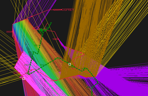
With lots of sensor data it can be increasingly difficult to determine which tracks should be made visible - the plot below shows just 12 visible tracks - it's possible to have many hundreds of tracks..
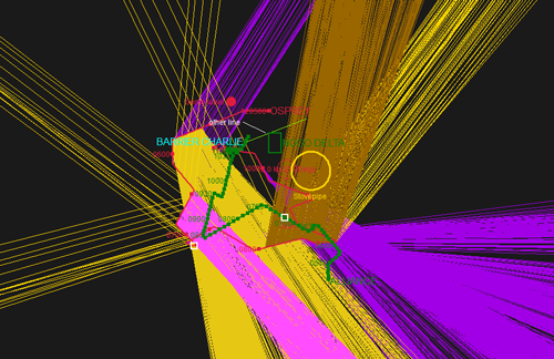
Cumbersome sensor data
The new Bulk Sensor Manager offers an opportunity to determine which sensor data has a direction near to one of the other tracks currently loaded in Debrief. Before opening the Bulk Sensor Manager it's worth telling Debrief which is your 'ownship' track, and which are the tracks of interest. Do this by marking tracks as primary and secondary in the Track Tote (see Section 4.1, “Assigning tracks as primary and secondary”). Once you have a primary track set, select Bulk Sensor Manager from the Window/Show View menu. You'll see a plot like the one below:
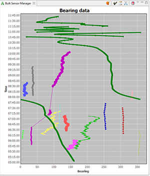
As you'll see, the view shows multiple series of track data. Currently visible tracks are displayed in bold lines (the thick green line in the screenshot) - so, you'll typically be trying to determine which blocks of sensor data are close to/similar to target tracks. Sensor data is shown with symbols if it's visible in the plot (see the pink line near the centre-left of the image). Clicking on a block of sensor data in the view also selects that sensor data in the Outline View (though on occasion you need to expand the Sensors folder in the Layer Manager). As blocks of sensor data are selected, they are shown in black in the view. Items can be multiple-selected with the <ctrl> key. Once multiple blocks of sensor data are selected in the Outline View you can right-click on them and select 'Merge sensors into xxxx'
Also note that whilst by default comes up with a unique color/symbol combination for each block of sensor data, you can click on the 'Show original colours' palette icon at the top of the view. This will switch the Bulk Sensor Manager to using the sensor data color as configured via the sensor manager.
For data from a command system that frequently 'wraps around' the track counter, when the data is read in Debrief will mistakenly assume that the data is all for the same contact: so the data will show as a continuous series to the left of the chart, then there'll be a jump over to were that track number is used again against another contact on the right hand side.
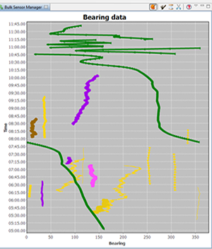
Debrief offers a tool to automatically split sensor data - the scissors icon at the top of the Bulk Sensor Manager offers 'Auto-split sensor segments'. It will pass through all of the sensor tracks in the primary track, and if there is a jump of more than 15 seconds Debrief splits the successive data into a new tracks. The original and new tracks are then renamed with a "_1", "_2" suffix.
In the above screenshot you can see that the purple dataset actually covers 3 periods of sensor data, roughly: 0545-0640, 0710-0720 and 0830-1010. If we click on the Axe toolbar button (
 , ), then we will see the tracks separated as in the following screenshot.
Sometimes the data extraction process results in sensor datasets being loaded/provided that cover time periods outside the range of the parent track. These unnecessarily slow down Debrief - so you may choose to delete them. The (
 ) operation will delete any blocks of sensor data that completely fall outside the time period of the primary track.
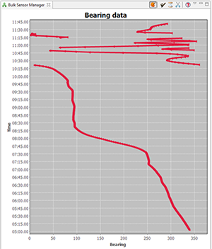
Sensor data loaded from a command system may contain many, many tracks. Many of the tracks will be of contacts unrelated to the platforms in question. It's quite easy for Debrief to determine sensor data that isn't related to the loaded secondary tracks. By clicking on the (
 ) button, Debrief will compare the bearing from the primary track to each secondary track. If a block of sensor data doesn't have a single cut that is within 45 degrees of any secondary track, it will be deleted. Running this operation on the above sample dataset gives this greatly reduced sensor dataset:
When very long sets of sensor data are exported to a report, it can be difficult for a reader to distinguish newer from old cuts - particularly when they are overlapping. Debrief provides support for this via the two operations:
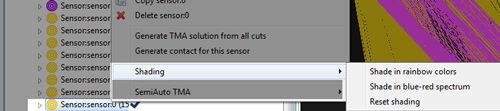
These two operations shade the selected block of sensor data (or whole sensor) according to two operations - as shown below.
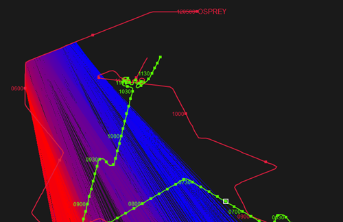
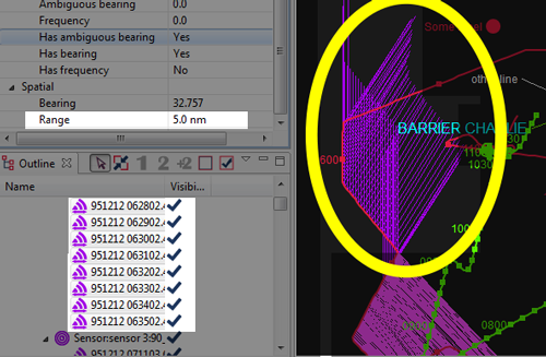
As you'll see in the earlier Cumbersome sensor plot, a lot of sensor data can make a plot difficult to interpret. If sensor data isn't provided with a range attribute, then sensor lines are drawn out to infinity (or the edge to the viewport - whichever is nearer...). On a large area plot this may given sensor lines of 10s of nautical miles long. If in truth the detections are only in the thousands of yards, you may wish to give the sensor data a range. To do this, start by multi-selecting a block of sensor data in the Outline View. Next, open the properties window - you'll see the elements have zero range. Just insert an 'indicative' value for range. The sensor lines on the plot will now be clipped to that range - greatly reducing plot clutter.
Trimmed sensor data
Whilst Debrief makes it easy to view a plot of the range between two vehicles, on occasion you may wish to view a time graph of the range from the array centre to the target. This graph can contain the distance from one or more sensors to a particular target. Open the graph by multi-selecting (<ctrl-click>) a series of sensor wrappers and a single target track (alternately you could select one track plus the 'Sensors' item of another track if you wish to view a range plot that includes all the sensors). If such a combination of objects have been selected in the Outline View, when you right-click on them you are offered the 'View sensor range plot' menu item:
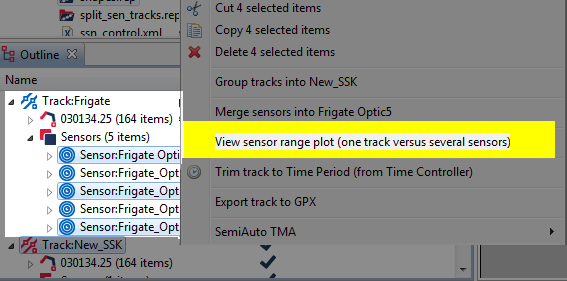
Popup menu with a track plus multiple sensor selected
Note, the Sensor Range Plot reflects the sensor offset length, plus whether the 'Worm in the hole' (see Section 11.1.3, “Worm in the hole”) property is set for each sensor.
![[Tip]](images/tip.gif) | Tip |
|---|---|
|
On occasion you may wish to view a sensor range plot of a sensor for which you haven't loaded sensor data. That is, you've loaded & displayed hull-mounted sonar data, but you wish to know the range from the centre of the array to the target. Do this as follows:
In this mode of use, the algorithm generates a range for each calculated position on the target track. In the normal mode (where we have sensor data), a range is calculated for each point at which there's a sensor cut (using interpolation to determine the position of the target track). |
![[Note]](images/note.gif) | Note |
|---|---|
|
Debrief is able to produce a plot of multiple sensors against on track, or the range from one sensor to multiple tracks - but it can't calculate the ranges for multiple sensors against multiple tracks. That would be just ridiculus. Your brain would explode, honest. |
Whilst hull-mounted sensor typically produce a single bearing to their contact, towed-arrays typically produce ambiguous bearings. They are aware of the relative bearing to the contact, but are now aware of whether it is to the Port or Starboard of the host platform.
The Debrief sensor format (DSF) handles ambiguous data by allowing two bearings to be read in, and once that block of sensor data is made visible Debrief plots both sensor bearings.
In order to analyse the sensor data, or use the sensor data in other analysis, the analyst must decide which is the actual bearing (to be kept), and which is the ambiguous bearing (to be removed).
Once a decision has been made on which of the two bearings to keep, open that block of sensor data in the Outline View. Then, select the relevant sensor cuts (using <shift> and <control> as necessary to multi-select). Once selected, right-click on one of the items and select or .
To support the display frequency residuals (as used in Section 12.2.3, “Dragging tracks”), Debrief contains a set of doppler frequency calculations (see Section 19.3.1, “Frequency algorithms”). Should you require this data in a third-party application it is possible to export this calculated data. Do this export as follows:
You must have a Debrief plot open that contains ownship plus target tracks
Ownship must be marked (Section 4.1, “Assigning tracks as primary and secondary”) as primary track (see Section 4.1.1, “Tote area”), and the target track must be the only secondary track
The ownship track must contain sensor data
The target track must have its base frequency assigned.
Using the Time Controller view (see Section 4.2.1, “The Time Controller”), select the time period for which data is to be exported
Select
The data is collated using the following algorithm:
Loop through the visible blocks of sensor data for the ownship track
Find all target track segments that overlap with this block of sensor data
Loop through this block of sensor data
For each sensor cut, find the position on the target track nearest to this time
Perform a doppler calculation for this sensor cut/target position
The data will now be written to file in csv format: first the base frequency then a series of time-stamped measured and predicted frequencies.
There exists the situation in frequency analysis where multiple tonals are held, but the analyst would rather use the highest freq tonals. Here's a strategy for how to manage it,
First, load the bearing sensor data. Edit the sensor cuts (probably in the grid editor, Section 3.8, “Using the Grid Editor”) to include the highest freq data held, potentially colouring the blocks of cuts according to the base tonal that they relate to. Go through these blocks of cuts creating a solution for each block - then setting the base frequency for that solution to the respective value.
You can now switch individual solution blocks on and off, ensuring the stacked dots (Section 3.1.3, “Track shifting”)will be working with the correct data values.
Should you have access to multipath sensor data of a target vessel from a host platform, Debrief is able to assist in determining the target depth. In overview, Debrief allows you to compare the measured time interval with one calculated from the relevant dispositions of the two tracks (plus measured sound speeds for that location).
To perform this analysis you require the following datasets:
Ownship and Target tracks
A SVP (Sound Velocity Profile) file for the location (using the file format defined in Section 16.5.2, “SVP file” ). The maximum depth of the SVP is interpreted as the depth of the water column: the depth slider is uses this value as its maximum, and it is used as the maximum permissible value in the optimisation algorithm.
A file of measured time intervals (using the file format defined in Section 16.5.3, “Time delays file”)
The indirect path length is calculated as follows:
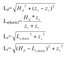
Algorithm used to determine indirect path length
Where:
Direct path length
Horizontal range to the point where the surface path intersects the surface (see diagram below)
Path length from source to surface
Path length from surface to receiver
Horizontal range
Source depth
Receiver depth
These lengths are the calculated as:
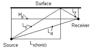
Comparison of acoustic paths
Finally the path lengths are divided by the respective sounds speeds to obtain the path travel times, and this the overall time delay:
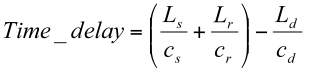
Calculation of time delay
The sounds paths shown in the illustration above may travel through depths that have varying sound speeds. We calculate an average sound speed for the depth profile by calculating a weighted mean for that depth range:
Source depth = 55 m
Receiver depth = 30 m
Sound Speed Profile:
| Depth (m) | Speed (m/s) |
| 0 | 1500 |
| 30 | 1505 |
| 40 | 1510 |
| 60 | 1515 |
Average sound speed between 0 m and 30 m can be ignored as the sound never goes into that region. Average sound speed between 30 m and 40 m is 1507.5 m/s. The sound speed at 55 m is 1513.75 m/s (through linear interpolation). Average sound speed between 40 m and 55 m is 1511.875 m/s. Using the depth range in metres as its weighting value, the overall average sound speed is ((1511.875*15)+(1507.5*10))/25 = 1510.125 m/s
Debrief is able to use Dr Michael Thomas Flanagan's (at www.ee.ucl.ac.uk/~mflanaga, [note: external link]) Nelder Mead simplex optimisation algorithm to determine the optimum target depth to minimise the least-squares error between the calculated and measured curves.
Perform multi-path analysis using the Multipath analysis view. Open this view by selecting it from the Window/Show View menu.
Initial view of multipath analysis view
As you'll see from the above screenshot, the panel is laid out with a series of controls above an xy plot. The controls at the top of the view indicate the files being used for SVP and time-delays, a slider control is provided to let you trial target depths, plus there's a magic button that runs an optimisation algorithm - generating a best-guess of target-depth by minimising the time-delay error.
So, start off by dragging in your SVP and time-delay files - dropping them over the respective [pending] label. Next, ensure your 'ownship' track is marked as the current primary track, and your target track is the secondary track in the Debrief Track Tote (as explained in Section 4.1.2, “Assigning tracks”).
Once you've loaded the data and assigned the tracks, the slider control will become enabled and you can drag it to trial new target depths. The xy plot will update to show a comparison of the calculated time delays against the measured delay. You'll determine the target depth estimate by using the slider to place the blue (calculated) line as close as possible to the red (measured) line.
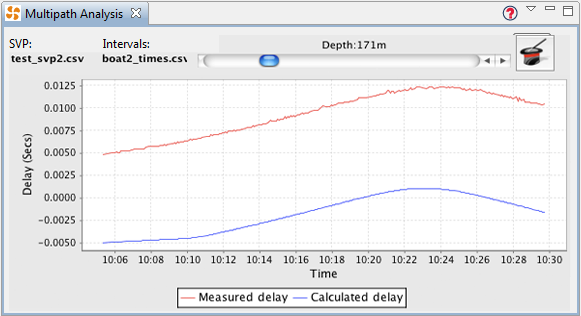
Multipath analysis view with data loaded
An alternative to working out the estimated target depth by eye/experimentation is to click on the magic top-hat icon. A Nelder and Mead simplex optimisation algorithm [note: external link] will now run - with the slider set to the result on completion. Should you be interested in the performance of this iterative optimisation algorithm, a summary of each step is placed as an information message in the error log (viewable by selecting //). The log will show the 'score' for each target depth trialled - normally only around 10-20 depths are necessary to reach an optimum.
Note, during development, on occasion the optimisation algorithm failed to produce a realistic target depth. On each occasion this was a symptom of there not being a valid result in the available target range (0 to 1000m) - which itself was symptomatic of invalid data files: dropping the data-files into the wrong 'slot' or mistakenly using units different to those specified in the reference (see Section 16.5.3, “Time delays file”).
| |  | |
| Chapter 11. Analysing sensor data |  | Chapter 12. Management of TMA and TUA solutions |